home

Loss functions, why?

July 2021

Notes:

Summary:

1. All loss functions merely give a way to optimize an objective; commonly, they are more than they appear to be.

2. Implicit and explicit biases riddle almost all objectives: Being aware of these is extremely important to understanding the model at a higher level

3. Some common loss functions secretly imply your errors lie within some distribution.

Comments:

1. These notes will assume you are intimately familiar with all forms of neural networks: ANNs, CNNs, LSTMs, RNNs, Transformers, etc...

2. These notes will assume you are intimately familiar with the optimization (the chain rule chain) of all of the above neural networks.

3. These notes will focus on intuition, as I believe that intuition is extremely important for this sort of work.

High level:

History and motivation:

Let’s start at the very beginning. What is a loss function? Usually, it’s some continuous and differentiable metric that allows us to numerically quantify the performance of the model. Lower the better.

As long as the loss function (LF) is continuous and differetiable, we can optimize the neural network using backpropogation and gradient descent. Gradient descent (GD) is the most common optimization algorithm for neural networks.

Why do we need LFs? Well, we need to optimize our models. We obviously can’t do a random search over the parameters, and we want some nice, smooth way to do it. LFs offer this.

What are these secret assumptions you say they make? There are many, but prior to discussing those, it’s important to note one high level idea: loss functions let you optimize the loss term, and nothing else.

Categorical cross-entropy (CE) on a discriminative classifier has no emotional investment in making your MNIST CNN work. More than that, optimizing CE doesn’t even inherintly make the accuracy go up. The loss function there only does what is stated in the formula. It’s important not to accidentally anthropomorphize loss functions.

The greediness of these loss functions is quite high, at times. Pathological edge cases are common, and in many cases, are actually the ideal state of the model. By realizing what your model is actually optimizing, you can understand and prevent these better.

I’d like to break the secrets of loss functions into 2 different groups: Secret MLE (SMLE), and secret side-effect (SSE).

SMLE is where a loss function directly stems from MLE, which is sometimes very sneaky.

SSE is an unintended (or intended) side effect of using a given loss function.

Medium level:

MSE and the Gaussian:

Let’s start with a nice and easy assumption some of you might not know: mean-squared-error (MSE) actually implies your residuals (your error) is Gaussian in nature.

You might wonder why, so I urge you to think about the formula for MSE. Why is it mean squared error, and not some other power? The squared is what ties it to the Gaussian.

How so? Well, recall MSE

\[\label{eq:mse} \frac{1}{N} \sum^N_{i=1} (y_i - \hat{y}_i)^2\]

and the Gaussian density.

\[\label{eq:normal} \frac{1}{Z} \exp \bigg( \frac{-( x - \mu)^2}{2 \sigma^2} \bigg)\]

Where \(Z\) is some normalizing constant we don’t really care about. Say you want to match some \(x_i\) to some \(y_i\) using a model \(f\), given a dataset of pairs. Now, assume your targets’ residuals are distributed according to a Gaussian. We can now write down the likelihood of \(y\) as:

\[\label{eq:likelihood} \mathcal{L} = \prod_i \frac{1}{Z} \exp \bigg( \frac{-(f(x_i) - y_i)^2}{2 \sigma^2} \bigg)\]

which implies:

\[\label{eq:loglikelihood} \log \mathcal{L} = \sum_i \bigg( \frac{-(f(x_i) - y_i)^2}{2 \sigma^2} \bigg) - \log Z\]

Now, since \(Z\) is secretly just \(\frac{1}{\sigma \sqrt{2 \pi}}\), if we assume \(\sigma\) is constant, our effective loss becomes:

\[\label{eq:real_mse} \log \mathcal{L} = \sum_i -(f(x_i) - y_i)^2\]

and if you look closely, you’ll see the first and last formula are in the exact same form, aside from a constant scaling.

This is the most simple example of SMLE.

An SSE of this is that outliers really, really ruin your loss. If your residuals are not gaussian distributed, but instead, bimodel: guassian with outliers, you can really have a bad time.

CE and KLD:

What about a categorical loss function, such as binary crossentropy-loss (BCEL)? Also a SMLE, that comes from an information theory idea called “cross entropy”.

The cross-entropy (CE) of a distribution \(q\), relative to a distribution \(p\), over a given set is defined as¹

\[CE(p, q) := H(p) + D_{\text{KL}}(p \vert \vert q)\]

where \(H(p)\) is the entropy of \(p\). For discrete probability distributions (such as the output of a softmax), \(p\) and \(q\), with the same support, \(\mathcal{X}\), \(CE(p, q) \equiv - \sum_{x \in \mathcal{X}} p(x) \log q(x)\)

What do these last two formulae actually mean, though? To understand that, we must look towards information theory.

The ‘Kraft-McMillan’ theorum states that:

Any (directly decodable) coding scheme for coding a message to identify one value \(x_i\) out of a set of possibilities \(\{x_1, ..., x_n \}\) can be seen as representing an implicit probability distribution \(q(x_i) = \big( \frac{1}{2} \big)^{l_i}\) over \(\{x_1, ..., x_n \}\), where \(l_i\) is the length of the code for \(x_i\) in bits.

meaning that CE can be interpreted as the expected message length when a distribution \(q\) is assumed while the data follows the distribution \(p\). In the case of \(q \equiv p\), this is merely the entropy of the random variable (and the optimal length). Minimizing CE can also be seen as minimizing the expected message length. When the divergence between \(p\) and \(q\) is minimal, the expected message length cannot be shortened beyond the entropy of \(p\)!

Given an observation of a random variable, \(x_i\), a corresponding binary label, \(y_i\), and a model, \(f\) parameterized by \(\theta\), with an output in the range \([0,1]\) that corresponds to a probability distribution, with \(f_\theta(x_i) = \hat{y} = p(y_i = 1 \vert x_i; \theta)\) and \(p(y_i = 0 \vert x_i; \theta) = 1 - f_\theta(x_i)\):

\[CE(p, q) = - \sum_i p_i \log q_i = -y \log \hat{y} - (1 - y) \log (1 - \hat{y})\]

Which optimizing directly corresponds to minimizing the KL divergence between the distribution output (\(f_\theta(x_i) \equiv q\)) and the true distribution (\(p\)), which, as stated previous, is just minimizing the expected message length.

Intuitively, this can be thought of as you wanting to make it so that the label of any observation (sample from \(q\)) can be communicated to an outside party in as few bits as possible. Obviously, we cannot communicate in less bits than the entropy of the random variable itself. However, we don’t know the true distribution (for if we did, we’d have a perfect classifier). So instead try to minimize the message length as much as possible.

You can generalize this to \(n\) classes directly by extending the support of the random variables.

An SSE of this is that optimizing the CE of a classifier doesn’t always lead to an increase in accuracy. Empirically, if you monitor validation accuracy of classification models, it will commonly at some point decrease as loss continues to decrease. This happens when the model is being incentivized to predict not only correctly, but correctly confidently. Accuracy has no concept of “confidence”, so sometimes this can lead to competing objectives.

GANs and JSD:

Let’s talk GANs. We all know and love them; a generator and a discriminator go at it in the Thunderdome™.

Put more seriously, GANs (generative adversarial networks) play a minmax game with the value function, \(V(G,D)\). The goal of the generator is to minimize it; the discriminator, to maximize it. This value function is a function of how well the generator ‘fools’ the discriminator.

Both the generator (\(G_\theta\)) and the discriminator (\(D_\phi)\) are usually neural networks, parameterized by \(\theta\) and \(\phi\) respectively. We set a prior (that we use as noise) for the generator, \(p(\mathbf{z})\), and represent a generator mapping between noise-space to data-space as \(G_\theta(z)\). We represent the discriminator mapping between data-space to the probability the generator generated that sample as \(D_\phi(\mathbf{x})\).

We then train the discriminator to maximize the probability of predicting correctly, while also training the generator to minimize the chance of the discriminator predicting correctly (to maximize the chance of the discriminated predicting a generated image as “real”).

This results in: \(\min_G \max_D V(D, G)= \underbrace{\mathbb{E}_{\mathbf{x} \sim p_{\text{data}} (\mathbf{x})}}_\text{A} \big[ \underbrace{\log D(\mathbf{x})}_\text{B} \big] + \underbrace{\mathbb{E}_{\mathbf{z} \sim p(\mathbf{z})}}_\text{C} \big[ \underbrace{\log (1 - D(G(\mathbf{z})))}_\text{D}\big]\)

1. A: A real sample of data is taken;

2. B: Since \(D(\mathbf{x}) \in [0, 1], \text{ } \log(D(\mathbf{x}) \in (-\infty, 0]\). Maximizing this corresponds to making sure the discriminator predicts real data as ‘real’.

3. C: A random sample of noise from our prior is taken.

4. D: Since \(D(G(\mathbf{z})) \in [0, 1], \text{ } \log (1 - D(G(\mathbf{z}))) \in (-\infty, 0]\) . However, this is the inverse of (B). Maximizing this corresponds to minimizing the probability the discriminator predicts fake data as real.

However, this hides the magic. Just taking this at surface level, it’s not easy to see why this would work, or what it’s truly even doing. We can intuitively say that this training will result in a generator that perfectly represents our true distribution, \(p_\text{data}\), but will it actually?

Let \(p_g\) represent \(G_\theta(z)\). Let \(p_\text{data}\) represent our true distribution. Let \(D^*_G(\mathbf{x})\) represent an ideal discriminator for fixed \(G\).

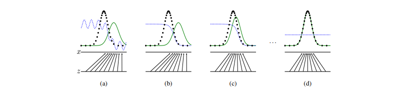
Figure 1. Discriminator: blue dotted line. Real distribution: black dotted line. Generator: solid green line. z represents our uniform prior. (a) shows a poorl fit discriminator and generator. (b) shows (a) after training the discriminator. (c) shows (b) after training the generator on the discriminator of (b). (d) is the end result of this back-and-forth.

Note that the training objective for D can be interpreted as maximizing the log-liklihood for estimating the conditional probability \(p(Y=y \vert x)\) where \(Y\) indicates whether \(\mathbf{x}\) comes from \(p_\text{data}\) (with \(y=1\)) or from \(p_g\) (with \(y=0\)). Our value function can then be written as:

\[C(G) = \max_D V(G, D)\] \[= \mathbb{E}_{\mathbf{x} \sim p_{\text{data}}} \big[ \log D^*_G(\mathbf{x}) \big] + \mathbb{E}_{\mathbf{z} \sim p(\mathbf{z})} \big[ \log (1 - D^*_G(G(\mathbf{z}))) \big]\] \[= \mathbb{E}_{\mathbf{x} \sim p_{\text{data}}} \big[ \log D^*_G(\mathbf{x}) \big] + \mathbb{E}_{\mathbf{x} \sim p_g} \big[ \log (1 - D^*_G(\mathbf{x})) \big]\] \[= \mathbb{E}_{\mathbf{x} \sim p_{\text{data}}} \bigg[ \log \frac{p_\text{data}(\mathbf{x})}{p_\text{data}(\mathbf{x}) + p_g (\mathbf{x})} \bigg] + \mathbb{E}_{\mathbf{x} \sim p_g} \bigg[ \log \frac{p_g (\mathbf{x})}{p_\text{data}(\mathbf{x}) + p_g (\mathbf{x})} \bigg]\] \[\mathcal{O} = \int_R p_\text{data}(\mathbf{x}) \bigg[ \log \frac{p_\text{data}(\mathbf{x})}{p_\text{data}(\mathbf{x}) + p_g (\mathbf{x})} \bigg] \text{dx}+ \int_R p_g (\mathbf{x}) \bigg[ \log \frac{p_g (\mathbf{x})}{p_\text{data}(\mathbf{x}) + p_g (\mathbf{x})} \bigg] \text{dx}\]

Due to the fact \(\int_R p(x) \text{dx}= 1\), we can add \(- \int_R p(x) \log [2] \text{dx}\) to both of the above integrals:

\[\mathcal{O} = - 2\log 2 + \int_R p_\text{data}(\mathbf{x}) \bigg[ \log \frac{p_\text{data}(\mathbf{x})}{p_\text{data}(\mathbf{x}) + p_g (\mathbf{x})} + \log 2 \bigg] \text{dx}+ \int_R p_g (\mathbf{x}) \bigg[ \log \frac{p_g (\mathbf{x})}{p_\text{data}(\mathbf{x}) + p_g (\mathbf{x})} + \log 2\bigg] \text{dx}\] \[\mathcal{O} = - \log 4 + \int_R p_\text{data}(\mathbf{x}) \bigg[ \log \frac{2 p_\text{data}(\mathbf{x})}{p_\text{data}(\mathbf{x}) + p_g (\mathbf{x})} \bigg] \text{dx}+ \int_R p_g (\mathbf{x}) \bigg[ \log \frac{2 p_g (\mathbf{x})}{p_\text{data}(\mathbf{x}) + p_g (\mathbf{x})}\bigg] \text{dx}\] \[\mathcal{O} = - \log 4 + \int_R p_\text{data}(\mathbf{x}) \bigg[ \log \frac{p_\text{data}(\mathbf{x})}{\frac{p_\text{data}(\mathbf{x}) + p_g (\mathbf{x})}{2}} \bigg] \text{dx}+ \int_R p_g (\mathbf{x}) \bigg[ \log \frac{p_g (\mathbf{x})}{\frac{p_\text{data}(\mathbf{x}) + p_g (\mathbf{x})}{2}} \bigg] \text{dx}\]

Recall the definition of Kullback-Leibler divergence:

\[\mathcal{D}_{\text{KL}}(P \vert \vert Q) := \int_R p(x) \log \bigg[ \frac{p(x)}{q(x)} \bigg] \text{dx}\] \[\mathcal{O} = - \log 4 + \mathcal{D}_{\text{KL}}\bigg(p_\text{data}\bigg\vert \bigg\vert \frac{p_\text{data}+ p_g}{2} \bigg) + \mathcal{D}_{\text{KL}}\bigg(p_g \bigg\vert \bigg\vert \frac{p_\text{data}+ p_g}{2} \bigg)\]

Recall the definition of Jensen-Shannon divergence:

\[\mathcal{D}_{\text{JS}}(P \vert \vert Q) := \frac{1}{2} \mathcal{D}_{\text{KL}}(P \vert \vert M) + \frac{1}{2} \mathcal{D}_{\text{KL}}(Q \vert \vert M)\] \[\text{with } M = \frac{1}{2} (P + Q)\] \[\mathcal{O} = - \log 4 + 2 \cdot \mathcal{D}_{\text{JS}}(p_\text{data}\vert \vert p_g)\]

Which means our value function objective really just minimizes the Jensen-Shannon divergence between the data generating process and the true distribution; yet another SMLE. Given an optimal discriminator and generator with sufficient capacity, \(p_g\) will converge to \(p_\text{data}\).

An SSE of this is that GANs are “mode seeking”, not “mode covering”. The GAN will happily not cover an entire mode of your distribution, as long as it can be better at other modes. For example, an MNIST generator may simply choose to only produce images of the digit “1”. As long as it generates these digits accurately, the discriminator has nothing it can do!

VAEs and ELBOs:

VAEs optimize the ELBO.

\[\text{ELBO} := \underbrace{\mathbb{E}_{q_\phi(z\vert x_i)}\bigg[\log p_\theta(\mathbf{x_i \vert z})\bigg]}_{\text{(A): Reconstruction likelihood}} - \underbrace{D_\text{KL} \bigg[q_\phi(\mathbf{z \vert x_i}) \vert \vert p(\mathbf{z})\bigg]}_{\text{(B): Prior constraint}}\]

Instead of starting at an idea and working towards a formula, let’s do the opposite. Let’s analyze what this objective is really optimizing.

(A) itself is very simple: we just want to maximize the probably to get the original sample from the encoders’ representation. Notice (A) doesn’t say how to do this; just merely what to do. In practice, BCE or MSE are usually used (by-pixel).

(B) is more nuanced, and has more interesting parts. A naive interpretation would simply be “keep the aggregate posterior near the prior", however, that’s missing a lot of the magic.

Recall that we use the reparameterization trick to allow low-variance gradient estimation. \(z \sim \mathcal{N}(\mu, \sigma) \equiv \mu + \sigma \cdot \epsilon, \epsilon \sim \mathcal{N}(0, 1)\). A side effect of this is that a single sample, \(x\), with fixed encoder parameters, \(\phi\), will almost never (probability 0) be represented in the same way twice. This fact encourages the decoder to reconstruct all samples within some small \(\delta\) of \(x\) to be reconstructed similarly. This is a major positive, as the decoder will have to learn to group together like samples.

In addition, (B) does one more major thing: it keeps all samples near the origin. This prevents the encoder from placing different representations arbitrarily far apart, which would make recreation possibly trivial.

An SSE of this is posterior collapse. If the model fails to optimize (A), it simply will optimize (B). How does it optimize (B)? Simply predict \(\mathcal{N}(0, 1)\) for every dimension of \(z\)! Ergo, the model output doesn’t even depend on the model input!

Takeaway:

Your loss function, almost agnostic of what you’re doing, should, at its’ core, be some simple objective. BCE is minimizing KLD. GANs just minimize JSD. VAEs just optimize the ELBO. And empirically? This just works.